Project Content → 30 Days Of Deep Learning Fundamentals

Github repo for today → Resnet_cifar10_pytorch

If you’ve been paying close attention, you probably have noticed that the models we have covered so far are not exactly new. The multilayered perceptron algorithms can be dated back to the late 70s. Alexnet from 2012 essentially marked the beginning of the recent deep learning boom in computer vision, and VGG gave us an answer to how deep a plain CNN can be. And that’s all before 2014.

Common models and their performance

So what followed after the year of 2014? Nothing much, but we have gone much deeper (In the arena of new network architectures. Developments in other areas are also worth mentioning, but I’ll skip it in this post.)

Alexnet from 2012 had 5 convolutional layers. The network took between 5 to 6 days to train on two GTX 580s. It may sound scary but remember Nvidia only debuted its consumer-level products of Maxwell (namely, GTX 900 series) in late 2014, and that is almost two generation old at the time of writing (Volta is now out on Titan, but still no GeForce yet.) Computational power has exponentially exploded since then. These structures can now be trained on your gaming PC for less than a few hours. In 2014 we also see VGG nets swept ImageNet 2014 competition. They varied in depths but the top performance came out from the VGG-16, which is a 16 layer architecture.

So how deep are we now? It might make your jaw drop. I still remember when I first took my neural network course in the 3rd year of uni (late 2015), the prof showed us a picture of the structure of GoogleNet. It was a whopping 22 layer network and the entire class was stunned by how deep it was. But take a look at what we have now. We have the four versions of Inception on one hand, with depths varying from several tens of convolutional layers. And then we have the monstrous 152 layer Resnet-152 on the other hand. Oh, how wonderful life is.

Blocks used in ResNet Left, a "building block" for ResNet-34 Right, a "bottleneck block" for ResNet-50/101/152

After digging around a bit, I decided to code up the Resnet architecture and see how good it performs on CIFAR-10/100 datasets. I’ll write a bit in Q&A about Inceptions.

Day 7

Focus of the day: Set up base code for cifar10 in pytorch

Tasks done

1. Study the difference between pytorch and tensorflow
2. Code up the base training code for CIFAR10/100

Q & A:

1. What is the difference between Pytorch and TensorFlow?

   The single most important difference is that Pytorch uses automatic differentiation while TensorFlow uses static computational graph (SCG). That means, in TensorFlow, you first define everything before you run the data through the graph. One of the pros of SCG is that it’s much easier to optimize. You can do tricks on a much lower level like preallocating resources and precompiling models. The cons are pretty obvious too: You practically can’t debug. It’s extremely cumbersome to debug in an SCG setting as the data is not there yet and you have no idea what could go wrong at runtime.

   Pytorch on the other hand, lets you debug like a breeze. Even if you don’t use an IDE or debugger, simply printing out the stack would probably help you catch any tiny bug you have written. Autograd is another mechanism that separates Pytorch and TensorFlow. Autograd is a define-by-run framework that’s used as the core of Pytorch differentiation logics. The backprop steps are defined by how the code is run, which means that every single iteration can be different, and you can change the model mid training.

   I may sound biased on this topic as a short answer won’t be able to cover all the pros and cons that these two frameworks have. I’d recommend an ML learner to use Pytorch simply because how easy it is to set up and get started. It’s also much easier to test out new models in Pytorch. TensorFlow is a production-ready framework that provides important features like distributed training and mobile device support. If you are not a learner, you may want to dig deeper and decides which to go for based on your use cases.

2. What is Batch Normalization?

   Batch Normalization Original Paper

   BatchNorm is a method of input normalization, refer to my last blog for what that means. It’s a technique to make the data inputs to any layer in a network “zero mean and unit variance”. The similar concept appears in data preprocessing and augmentation too.

   So why is “zero mean and unit variance” a good thing? By having a fixed distribution of input data, we effectively eliminate the problem of forcing the layers to continuously adapt to new distribution during training. When the distribution to a specific layer changes, it could slow down the training by requiring lower learning rates and saturating non-linearities.

   In short, BatchNorm enables faster training and potentially improve the performance of a model.

   I decided to test it out, and the results are exactly like what the paper claimed.

   

   Orange line: ResNet-18 Grey line: ResNet-18 without BatchNorm

   

   Red line: With BN top1 performance Orange line: Without BN top1 performance

   Here’s the step-by-step list of operations of how you do a BatchNorm.

   

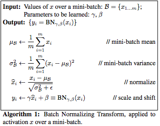
   It may be really confusing if you are looking at the list for the first time. The original paper has given some intuition behind it, but if you still find it hard to comprehend, I recommend the video lectures from Andrew’s course on Coursera.

3. Batch Norm vs Dropout?

   Simply put, when using the dropout technique, you intentionally ignore a randomly selected set of neurons during a certain iteration of training process. At each iteration of training, each node is either dropped or preserved with a pre-set possibility of P (usually a number somewhat around 0.5, which means a 50% dropout rate.)

   Dropout is a training regularizer, it prevents overfitting and regularizes the network. Batch Norm is an input normalizer, it’s mostly about improving optimization and “stabilize” the network. Usually, overfitting won’t be a huge problem if you have a large enough dataset. Then optimization has a higher priority in this kind of scenarios. But when you have a relatively small dataset or overly complicated network, you will have a higher risk of overfitting the model. Then it won’t matter how faster or well you train (which is improved by using optimizing techniques), the performance of your model will be capped by overfitting.

   Although BatchNorm is an input normalizer, in practice, people often find it also helps regularize the training as well. You can safely reduce the strength of the dropout in your network or even remove it when you are using BN. If you still find overfitting behaviour in training, try to increase the strength of your regularizers and it would help.

Day 8-9

Focus of the day: Code up the ResNet models

Tasks done

1. Code up the ResNet models

Q & A:

1. What is data augmentation and preprocessing and is it helpful?

   These two terminologies might look rather similar. Isn’t data augmentation a type of data preprocessing? Some may even argue the other way around: isn’t preprocessing a method of data augmentation?

   In general, by “data preprocessing”, we mean the process of reducing the noisiness in data and in turn improve the quality of data. By data augmentation, we normally mean to improve the training performance by artificially inflating the size of data with various techniques. But I’ve also seen counter-examples where people simply use them interchangeably. For example, in Keras, all related operations are under the class “preprocessing”.

   Let me give you some quick examples of what these two concepts refer to. When you are performing an image classification task, you can normalize the input data by making the mean(average) of your data zero and variance 1 (This is called zero-mean-unit-variance data normalization). You can easily see why this would work. By regulating the distribution of the input data, we artificially made the task easier for the classifier we are about to train. This is usually referred as a way of image preprocessing.

   On the other hand, data augmentation emphasizes the “augmentation” part. For example, in image related tasks, you often can inflate the size of your dataset by manually rotate/flip/crop your images and feed them into the training process along with your original images. If you rotate a picture of a potato, your classifier should still recognize it as a potato, and if you flip a cup, your classifier should still be expected to classify the cup as a cup. That’s basically the reasoning behind data augmentation.

   Believe me, this actually has a huge impact on the performance of your model. In the last post, I trained a VGG16 model on the CIFAR10 dataset. It was a 5% - 7% drop in TOP-1 accuracy if I do nothing with the data. It’s extremely important in Computer Vision as it’s often times pretty low-cost to generate synthetic data and they resemble the real-world variations really well.

2. What’s training regularization?

   Regularization, as defined in Ian Goodfellow’s book, is “any modification we make to the learning algorithm that is intended to reduce the generalization error, but not its training error.” This definition is quite broad. So broad that it even counts data augmentation as a form of regularization. In general, when we talk about regularization, we refer to a range of techniques that help regularize the training process to prevent common pitfalls like overfitting. Some of the most common techniques include weight decay, dropout layer and early stopping.

3. What are deep ConvNets learning?

   Here you go, a video from Andrew’s lecture on coursera.

   You can always get a pretty intuitive visualization by outputting the hidden layers in a ConvNet.

   What a deep ConvNet does is that it extracts “features” from the input. A feature is a specific region in the input that represents a piece of information that may help solve the computational task. What a feature extractor does is that it reduce the amount of information in the original data (an image, in our case), and derive a set of values(features) that is informative and non-redundant. For example, feed an image of a city scene into a feature extractor, the features it extracts may be things like cars, people, trees, buildings, etc.

   Lower layer in a deep ConvNet looks at a smaller region and more detailed features. The first layer is usually activated by lines in different angles. The second layer may start to look at shapes. The deeper it goes, the more concrete the features are and the larger an area it looks at. As the video from Andrew’s lecture, the trained network already started to look for wheels and dog faces starting from the fourth layer.

Day 10

Focus of the day: Adjust the hyperparameters and test model performances

Tasks done

1. Try different sets of hyperparameters and depths of models, record the performances
2. Case study: Residual network vs Inception network

Q & A:

1. What’s inception network?

   [Original Paper: Going Deeper with Convolutions]

   As you can guess it’s just another deep learning architecture, but not simply “just another deep learning architecture”.

   Inspired by Network in Network by Lin et al., The authors proposed a network architecture that’s composed of these “Inception modules”.

   

   Inception modules

   The whole theme of “Deep Learning” is basically to go as deep as one can without exhausting the computational power that one possesses, and the trend of increasing the number of layers and layer sizes never stopped. But the problem is, around the year of 2014, when we’ve seen architectures like VGGs coming out, people found that it is unsustainable to simply stack layers on top of each other.

   In a deep vision network, if two conv layers are chained, any uniform increase in the number of their filters results in a quadratic increase of computation. If the added capacity is used inefficiently (for example, if most weights end up to be close to zero), then a lot of computation is wasted.

   The fundamental way of solving both issues would be by ultimately moving from fully connected to sparsely connected architectures, even inside the convolutions.

   And that’s exactly how inception modules solve the problem. The main idea of the inception architecture is based on trying to find out how an optimal local sparse structure in a convolutional vision network can be approximated and covered by readily available dense components.

   In the above graphs of the structures, the naive version is what the authors think a module should look like. It uses multiple filters of different sizes to produce various features of different scales. It then concatenates the outputs and feeds the result into next layer.

   Another practically useful aspect of this design is that it aligns with the intuition that visual information should be processed at various scales and then aggregated so that the next stage can abstract features from different scales simultaneously

   The problem with the naive version is that even a small number of 5x5 convolutions can be extremely expansive if it’s placed on top of a large number of filters. What makes the problem worse is that the pooling layer will output the same number of filters as the previous stage, which means the number of filters will only grow. This would soon lead to what the authors call a “computational blow up”.

   The problem is solved by introducing 1x1 convolutional layers. It effectively reduces the number of filters by convolving the input with 1x1 convolutional filters. Because it’s topped with a ReLU activation, it also induces more non-linearity. The final structure of inception modules look like this:

   

   Architectures like ResNet and Inception helped break the computational barrier and can be used to build much deeper neural networks.

2. What is the difference between each version of Inception?

   You have to admit Christian, who is the lead author of the Inception series, is quite productive and dedicated. In the short span of roughly two years, he published two follow-up papers of the Inception architectures and now we have a total of 4 versions of Inception networks.

   Inception v1: Going Deeper with Convolutions
   Inception v2 & v3: Rethinking the Inception Architecture for Computer Vision
   Inception v4: Inception-v4, Inception-ResNet and the Impact of Residual Connections on Learning

   You can refer to the papers if you want detailed explanation behind each update to the model. I’ll give short one line descriptions of the differences between each version here:

   v1 -> v2: Factorization. Breaking large convolutional filters into small ones.
   v2 -> v3: Add BN-auxiliary.
   v3 -> v4: Add residual connections similar with the ones in ResNet.